Reversibility of Climate Change Impacts on the Marine Environment

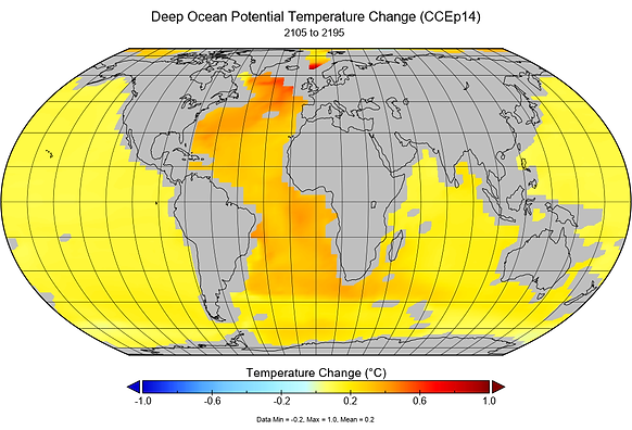
Figure 1: This map shows that warming in the deep ocean will continue well after society experiences a simulated 'overshoot' of CO2 emission targets, but returns to them by 2100 via net negative emissions.

Introduction

Humanity is on track to bypass the emission target set by the Paris Agreement to limit warming to well below 2°C. This makes it more likely that technologies that can remove CO2 from the atmosphere, will be needed in the future to reverse emission overshoots occurring now. Studies have shown that active removal of CO2 from the atmosphere is effective at reversing temperature change from CO2 emission overshoot scenarios on centennial time scales (Toarska & Zickfeld, 2015). However, studies also indicate that changes to certain aspects of the climate system, such as that of ocean acidification, will be more difficult to reverse. In particular, deep ocean response to climate change has been stated to be slow, meaning impacts occurring now can persist for centuries even after emissions reversal.

We explore these concepts and whether the reversing of atmospheric CO2 concentration following an ‘overshoot’, can reverse the impacts it has on the ocean. We compare the response of the surface ocean to the deep ocean following these scenarios.

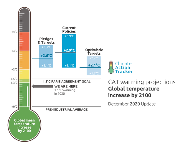
CAT-Thermometer-2020.12-3BarsText.width-

Figure 2: The December 2020 update on warming target goals by the Climate Action Tracker, shows we are well off track of the 1.5°C Paris goal and will close in on 3.0°C of warming by 2100 if nothing more is done.

Source: https://climateactiontracker.org/

Methods

This study uses the University of Victoria Earth System Climate Model (UVic ESCM), which is a coupled climate-carbon model of intermediate complexity to run four simulations. The first being a historical plot showing observed CO2 emissions from 1800 to 2000. The other three are described as Cumulative Constant Emissions (CCE) scenarios, which are defined by an identical total emissions amount of 551 gigatons of carbon from fossil fuels and land use change. The simulations are run from 2001 to 2500, with the total cumulative emissions target reached by 2200.

The scenarios are listed as follows:

1. Historical data showing observed CO2 emissions from 1800 to 2000.

2. "CCEp10" has CO2 emissions capped at a level that limits warming to 2°C, with no overshoot and thus no negative emissions required.

3. "CCEp12" has slight overshoot of CO2 emissions and subsequent removal of CO2 to reach the same emissions target.

4. "CCEp14" experiences the largest overshoot and a greater amount of net negative emissions to return to the emissions target.

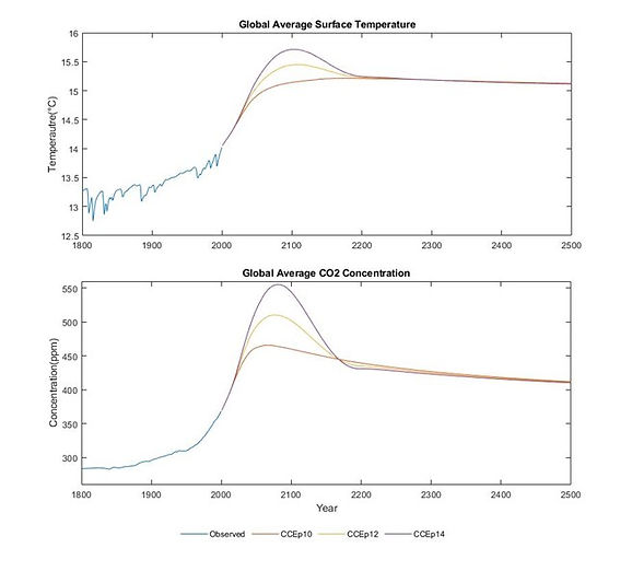
Figure 3: Changes in temperature and CO2 concentration plotted against time in years. The blue plot indicates the historical simulation from 1800 to 2000, CCEp10 is in orange, CCEp12 is in yellow and CCEp14 is in purple. As we are removing CO2 in the overshoot scenarios to limit warming, all CCE scenarios show approximately equivalent CO2 concentration around year 2200.

Results

Surface

Total (Deep)

We compared variables that have major implications on ocean processes and marine environments, comparing the responses of these variables between the surface and ocean and the total ocean.

Surface Ocean

With the exception of surface alkalinity, all other surface variables, temperature, oxygen concentration, and surface dissolved inorganic carbon (DIC), can be reversed to the same level as the scenario without an 'overshoot', following net negative emissions over the period 2100 to 2200 (Figure 3 graphs a ,c, e, g). These results largely match the atmospheric CO2 concentration and temperature trend, as surface ocean temperature, oxygen and dissolved inorganic carbon (DIC) display a similar dependence on cumulative emissions, which largely controls the responsiveness of the surface ocean to changes in the atmosphere. Processes that affect climate change impacts on the surface ocean operate on decadal timescales which can initiate a relatively quick response of the surface, to changes in the atmosphere.

Total Ocean

The total ocean conditions are not reversible in the studied time scale. With the slowly, but steadily rising temperature, the average oxygen concentration will continue to decrease and DIC will continue to increase (Figure 3 b, d, f, h). This is due to the longer timescales associated with deep ocean processes, as well as the increased stratification and reduced circulation as a result of higher temperatures and lowered solubility. This makes it much harder for changes happening at the surface to reach or influence the deep ocean quickly.

Note on alkalinity and model limitations

Most studies include the response of pH to changing CO2, but the response of alkalinity or the ability for the ocean to buffer pH change is measured here instead. Our result of a consistent decrease in alkalinity goes against studies that suggest alkalinity will instead increase due to reduced biogenic calcification and thus reduction in precipitation of CaCO3 out of the surface and into the deep ocean (Egelston et al., 2010). However, some studies suggest other controls on the total alkalinity may play a role, including the thermal expansion of the ocean to reduce overall concentration and the freshening of the ocean that causes a reduction in alkalinity (Fine et al., 2017).

The simulations run here are based on variables measured from a single model and are subject to parameterization and uncertainty in processes specific to the UVic model used. The variables measured also represent the averages of the surface and the total ocean respectively and differences found, primarily in alkalinity, are likely due to the model’s specific simulation of the processes that affect it.

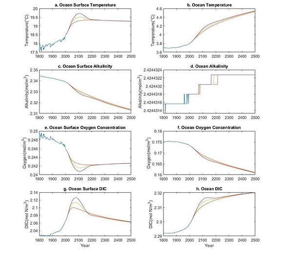
Figure 4: Displayed are graphs of each ocean variable simulated for each scenario. They are plotted for the surface ocean and total ocean for comparison. Most notable are the recovery of the surface temperature, oxygen concentration and dissolved inorganic carbon (DIC) to a consistent value regardless of emissions overshoot. In contrast the total ocean temperature, oxygen and DIC vary less between each scenario and largely continue the trend they were on before the simulations began.

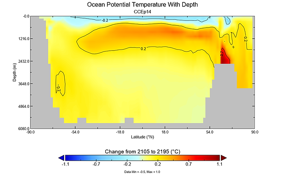
Figure 5: This depth chart shows that between 2105 and 2195 when net negative emissions are being simulated, the surface ocean cools while the rest of the ocean continues to warm. This supports the idea that climate change impacts occurring in the deep ocean are significantly lagged behind those occurring at the surface.

Conclusion

Our findings agree with what was found by Mathesius et al. (2015) and Cao et al. (2014), that climate change impacts will continue to be seen in the deep ocean long after the cessation of emissions or removal of emissions. This is in contrast to the changes that occurred in the surface ocean being shown to be largely reversible following net negative emission scenarios. The convergence of deep ocean variable trends onto a similar constant value indicate the independence of these variables on scenario taken, but rather are controlled by the cumulative emissions amount. Thus, the values presented for variables in the deep ocean may only be affected if this cumulative emissions value is changed. This presents an incentive on society to begin reducing emissions sooner rather than later, because the more we emit cumulatively, the greater the change that will eventually be felt in the deep ocean. According to our study and others discussed, this change will be irreversible over human timescales regardless of future CO2 removal attempts. However, if the changes in the surface ocean can be reversed from CO2 emissions overshoots, then it can be assumed that the impacts caused by even greater emissions than the highest scenario we measured should be reversible.

UVIC model: (Eby et al., 2009; Weaver et al., 2001)

CCE scenarios: (Tokarska & Zickfeld, 2015)

Graphs and maps created in MATLAB using data from the UVic ESCM.

Project created by Riley Smith and J.. Kim in Spring 2019 for GEOG 414 Climate Change at SFU. Acknowledgments to teaching assistant C.M. Nzotungicimpaye and Dr. Zickfeld for helpful comments and direction.

References

Cao, L., Zhang, H., Zheng, M., & Wang, S. (2014). Response of ocean acidification to a gradual increase and decrease of atmospheric CO2. Environmental Research Letters, 9(2), 024012.
Eby, M., Zickfeld, K., Montenegro, A., Archer, D., Meissner, K. J., & Weaver, A. J. (2009). Lifetime of anthropogenic climate change: millennial time scales of potential CO2 and surface temperature perturbations. Journal of Climate, 22(10), 2501-2511.
Egleston, E. S., Sabine, C. L., & Morel, F. M. (2010). Revelle revisited: Buffer factors that quantify the response of ocean chemistry to changes in DIC and alkalinity. Global Biogeochemical Cycles, 24(1).
Fine, R. A., Willey, D. A., & Millero, F. J. (2017). Global variability and changes in ocean total alkalinity from Aquarius satellite data. Geophysical Research Letters, 44(1), 261-267.
Mathesius, S., Hofmann, M., Caldeira, K., & Schellnhuber, H. J. (2015). Long-term response of oceans to CO2 removal from the atmosphere. Nature Climate Change, 5(12), 1107.
Tokarska, K. B., & Zickfeld, K. (2015). The effectiveness of net negative carbon dioxide emissions in reversing anthropogenic climate change. Environmental Research Letters, 10(9), 094013
Warming Projections Global Update December 2020 (2020). Climate Action Tracker. Retrieved from https://climateactiontracker.org/documents/829/CAT_2020-12-01_Briefing_GlobalUpdate_Paris5Years_Dec2020.pdf
Weaver, A. J., Eby, M., Wiebe, E. C., Bitz, C. M., Duffy, P. B., Ewen, T. L., ... & Meissner, K. J. (2001). The UVic Earth System Climate Model: Model description, climatology, and applications to past, present and future climates. Atmosphere-Ocean, 39(4), 361-428.